Inference

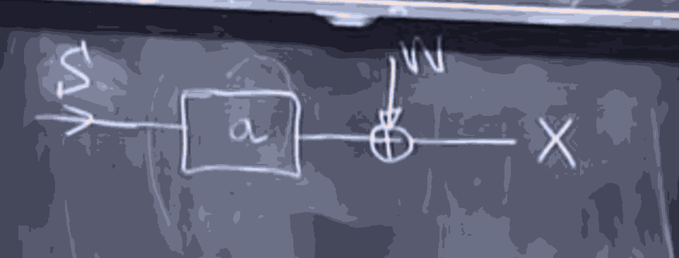
So we have some signal $S$ going through a box which does something "deterministic", and turns $S\mapsto f(S,a)$, where $a$ is some collection of parameters, and then some sort of noise $W$ is applied, to get the final output, So we can say $X=g(f(S,a),W)$. Where $f$ is a process that we actually know. but intead of getting the result directly from $f$, there is some Noise $W$ being applied by $g$. (we don't know $g$).

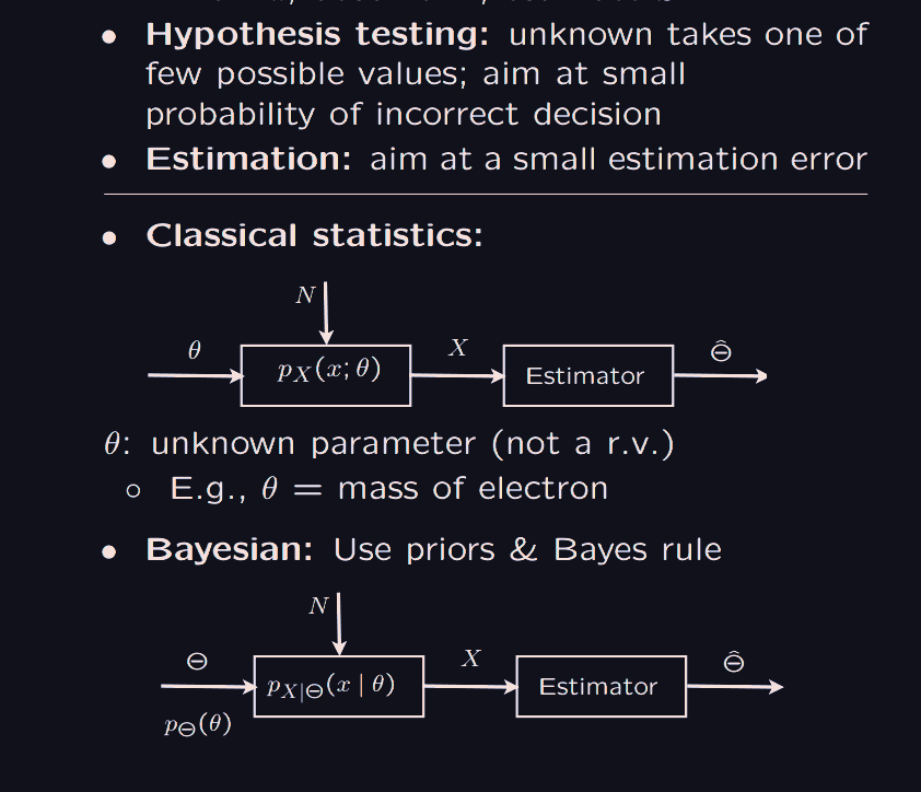
Then there are two types of inference problems:

• Where we can see both $S$ and $X$, and use it to estimate the parameters $a$, of the box $f$, dealing with the noise applied by $g$.
• Where we know the parameters $a$, And we can measure the output (noisy) signal $X$, and try to figure out what $S$ went inside.

So HWEN we have a finite set of possibilities for the unknown, we have to make a decision with least probability of error. (Hypothesis testing)
if the unknown is on a continuum, we aim at a small estimate error. (Estimation)

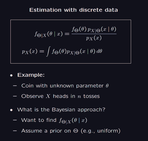
Let us talk about estimating the mass of electron. Of course the mass of the electron $\theta$ is not a random thing, it is a constant.
Imagine we have a noisy measuring apparatus, that takes in the mass of the electron and gives out a measurement modelled as a random variable $X$.

In classical statistics, The model of the measuring apparatus, is a probability distribution of $X$, which is of course affected by the mass of the electron $\theta$ and some noise. So in classical statistics, we are thinking of measuring apparatus, as simply putting a distribution over the noisy measurement of the mass of the electron.

The Bayesian philosophy is that even though the mass of an electron is constant, what we DONT KNOW, we should put a distribution on it. so $p_{\mathrm{\Theta }}$ is some "prior" distribution on $\theta$, which if we don't know ANYTHING we might say, all masses of the electron in a certain range are equally likely, or we can put a more sophisticated prior distribution $p_{\mathrm{\Theta }}$ on $\theta$, based on previous work.

The model of our measurement box, is a distribution of the random variable $X$, given the random variable $\mathrm{\Theta }$, with distribution $p_{\mathrm{\Theta }}(\cdot )$.

The "new and better" random variable that we need to put a distribution on, is actually $\mathrm{\Theta }|X$ (posterior distribution), because if we had some "prior" belief on the distribution of $\mathrm{\Theta }$, and out measuring box, gives us the distribution of the output data $X$ conditioned on the distribution of $\mathrm{\Theta }$, We hope that when our prior belief on $\mathrm{\Theta }$ improves to a better belief, after conditioning it on the output data $X$.

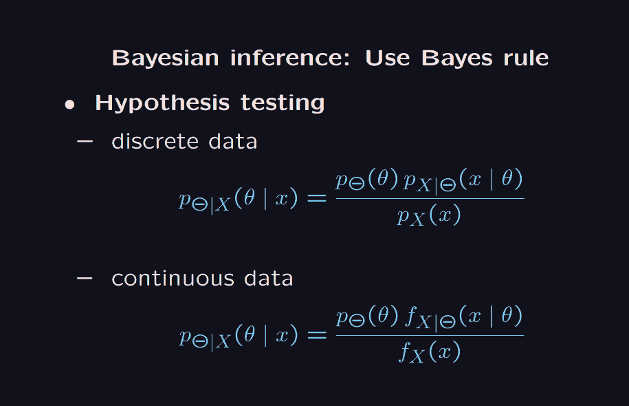
Bayesian hypothesis testing and estimation

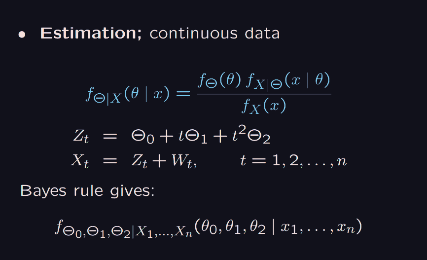
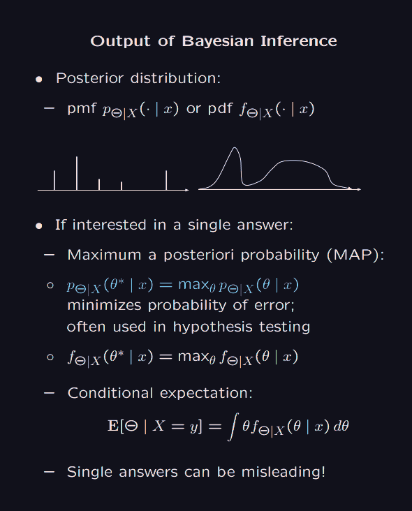
So in this picture, $Z_t$ is the height of a bird at time $t$. We believe it to be parabolic, and so we want to estimate the coefficients. So we have some prior beliefs on these coefficients (as random variables), and we make measurements at $n$ time steps, modelled by the random variable $X_t$, unfortunately, the measurements are noisy, so we think that $X_t$ is equal to $Z_t$ plus some pure noise random variable $W_t$. And if we have a reasonable idea of what distribution to put on $W_t$, and hence infer the distribution on $X_t$, We have all the data, to use the bayes rule, to UPDATE out belief of the distribution on the priors ${\mathrm{\Theta }}_1,{\mathrm{\Theta }}_2,{\mathrm{\Theta }}_0$, to the posterior belief (after seeing some data) which has the distribution shown in the above picture.

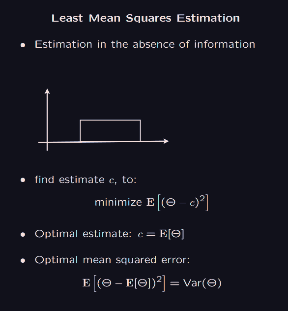
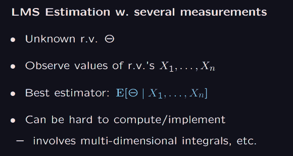
Least mean square estimation

In the above picture, we have no information more about $\mathrm{\Theta }$,
and we want to estimate it with a single real number $c$.
We can do this by minimized $E[(\mathrm{\Theta }-c{)}^2]$, which using calculus, we get $c=E[\mathrm{\Theta }]$. So if our goal to minimize the expected squared error (or mean squared error) between a random variable and an estimate, we best set the estimate to the mean of the random random variable.

Now, let us introduce some extra information, and say that a measuring device, that noisily measures $\mathrm{\Theta }$ outputs the random variable $X$.
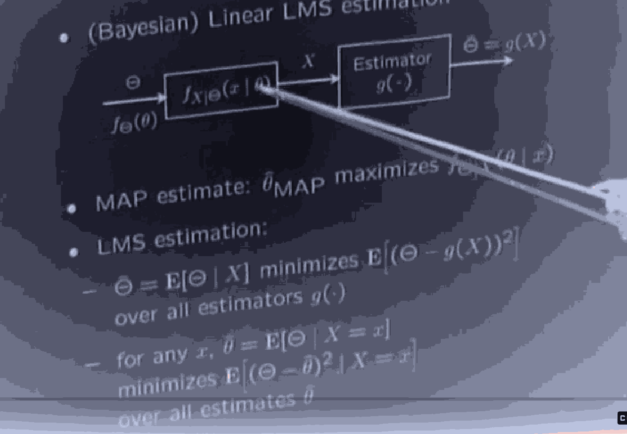
So then, in the usual Bayesian way, we want an estimate $g(X)$, which is a random variable, that whenever we see that $X=x$, we think $g(x)$ is a good estimate for $\mathrm{\Theta }$.

Basically what we are saying, is that given the data $X$, whenever $X=x$, we want to minimize the posterior error $E[(\mathrm{\Theta }-g(x){)}^2|X=x]$. The function $g$ is called an estimator, because based on the random variable $X$, and whatever value we observe from it, it gives an estimate of $\mathrm{\Theta }|X=x$.

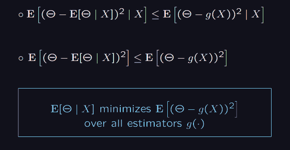
Now, the question is, could there be an estimator of the posterior $\mathrm{\Theta }|X$ that has the least mean squared error, no matter what value $X$ collapses to?

When, Let us use the arbitrary choice of $x$ technique to show that there is global best estimator.

Well, pick arbitrary value $x$ that $X$ collapses to. In this new (and fixed) conditional universe, we want to minimize $T=E[(\mathrm{\Theta }-c{)}^2|X=x]$. Expanding it out: $T=E[{\mathrm{\Theta }}^2|X=x]+c^2-2cE[\mathrm{\Theta }|X=x]$, Again taking the derivative of $T$ wrt to $c$, and setting it equal to zero, we get that the best $c$, is actually just $c=E[\mathrm{\Theta }|X=x]$.

So no matter what $x$ we pick, for that $x$, the least mean squared estimate for $\mathrm{\Theta }|X=x$ is just $E[\mathrm{\Theta }|X=x]$.

Which means that for any estimator rv $g(X)$ of the unknown $\mathrm{\Theta }$, given data $X$, is actually the random variable $E[\mathrm{\Theta }|X]$.

So we have concluded that the best estimator (or bestimator), in the besian setting: of having some unknown $\theta$, modelleled by the random variable $\mathrm{\Theta }$, and some prior distribution $f_{\mathrm{\Theta }}(\cdot )$, and a noisy measurement modelized by $f_{X|\mathrm{\Theta }}$, which outputs measurements, which are modelled by the random variable $X$, where we update out prior distribution on $\mathrm{\Theta }$ to a better posterior distribution, on $\mathrm{\Theta }|X$ using the bayes rule.

So the best estimator $g(X)$ in this setting, which minimizes expected squared error between $\mathrm{\Theta }$ and $g(X)$ in the universe conditioned on the random variable $X$, is $g(X)=E[\mathrm{\Theta }|X]$.

And furthermore, it is not only true that $E[\mathrm{\Theta }|X]$ beats out any other $g(X)$ (for LMS error) in the universe conditioned on $X$, but it beats out any estimator $g(X)$ in general.

That is, for some observed data modelled by $X$, The estimate $E[\mathrm{\Theta }|X]$ for $\mathrm{\Theta }$ itself, in the conditional universe, is a better estimate than any other function $g(X)$ on the observed data.

We write this estimator $E[\mathrm{\Theta }|X]$ as $\hat{\mathrm{\Theta }}$.

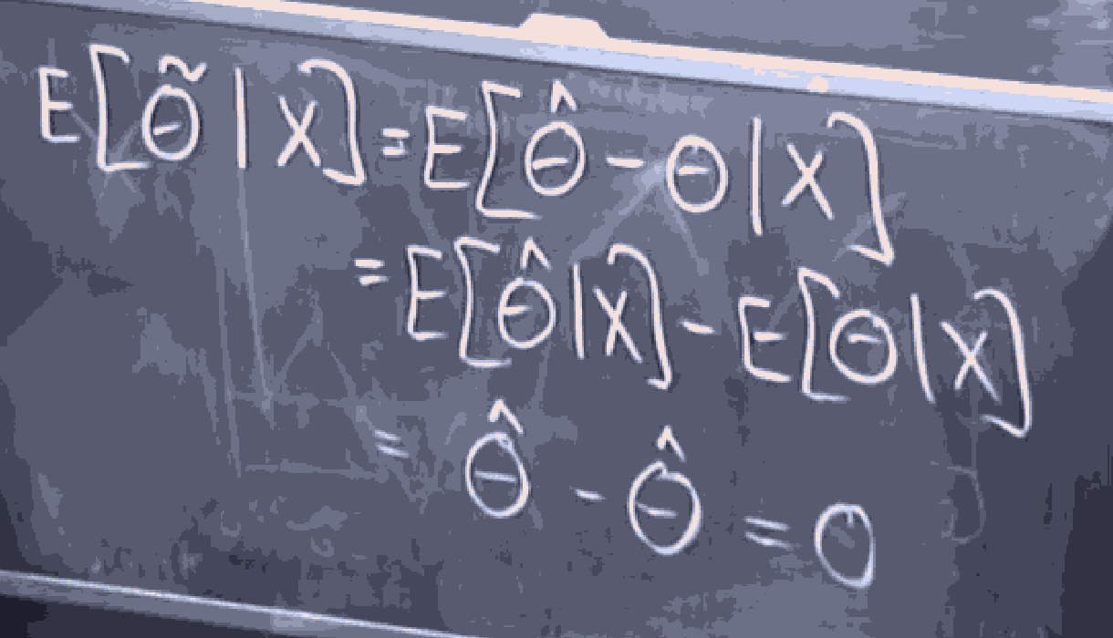
So HWAT IS THE ERROR OF THIS ESTIMATOR? well, its $\tilde{\mathrm{\Theta }}=\hat{\mathrm{\Theta }}-\mathrm{\Theta }$. what is the expected value of this error

The above idea comes from the fact that $\hat{\mathrm{\Theta }}=g(X)$, hence $E[\hat{\mathrm{\Theta }}|X]=\hat{\mathrm{\Theta }}$, (when we give the random variable $X$, $\hat{\mathrm{\Theta }}$ is determined, hence its expected value is itself), and also by definition $\hat{\mathrm{\Theta }}=E[\mathrm{\Theta }|X]$.

So my expected error between the bestimator and the unknown random variable, conditioned on any data, is the random variable $O$. (zero)

That is $E[\tilde{\mathrm{\Theta }}|X]=O$. Notice that this expectation is actually a function on the random variable $X$. if no matter what $x$ you pick, this function takes it to $0$, then the expected value of the error (unconditioned) $E[\tilde{\mathrm{\Theta }}]=0$ (the the number 0).

Now, notice that $E[\tilde{\mathrm{\Theta }}h(X)|X]=h(X)E[\tilde{\mathrm{\Theta }}|X]=O$. Hence, no matter what the random variable $X$ is, the expected value, $E[\tilde{\mathrm{\Theta }}h(X)]=0$ (the number zero).

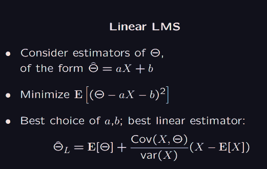
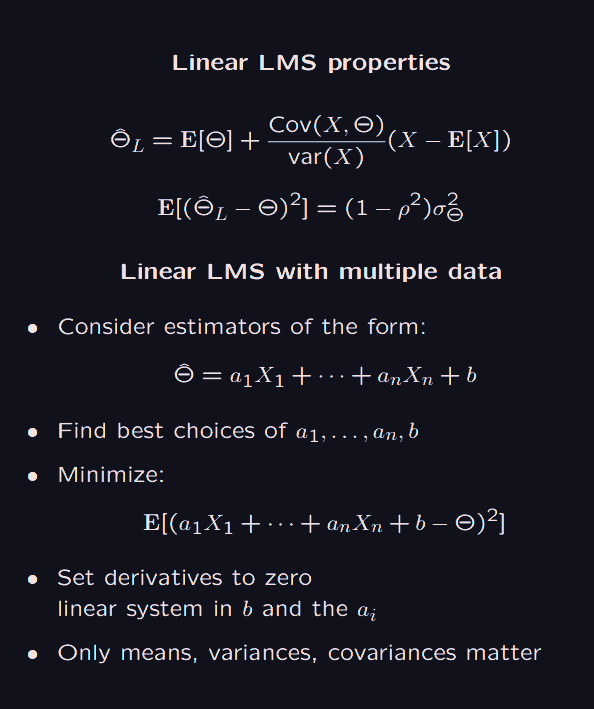
Now for the linear LMS, we assume our estimator to have an affine relationship with the data variable $X$

There is some nice intuitive idea here. Of course, given a prior on $\mathrm{\Theta }$, we start with the mean(or expectation) of this prior.
Then, given the data $X$, we look at the covarience of $\mathrm{\Theta },X$.
If the data we collected has no covariance (covarience is zero) then the data we collected is useless. Hence the mean of the prior is still the best we can do.

if covariance of $\mathrm{\Theta },X$ is positive, they both are bigger than their means, or smaller than theirs means together, respectively. In this case, for some observation $x$ if it was bigger than the mean $E[X]$, then the $\theta$ that came in, was probably bigger than it's own mean, and because co-variance is positive, this is what actually happens, we add something to $E[\mathrm{\Theta }]$. And the other way around works too, whenever $x$ is smaller than its mean, since covarince is positive, we are taking a little away from $E[\mathrm{\Theta }]$

if covariance of $\mathrm{\Theta },X$ is negative, then an analogous argument can be made.

So we are making corrections on our prior, based on the covariance of the data and the prior.
The error of this linear estimator, increases when the prior itself is quite uncertain, that is, ${\sigma }_{\mathrm{\Theta }}^2$ is large. And the error gets smaller when the correlation $\rho$ between $X$ and $\mathrm{\Theta }$ has a large magnitude.

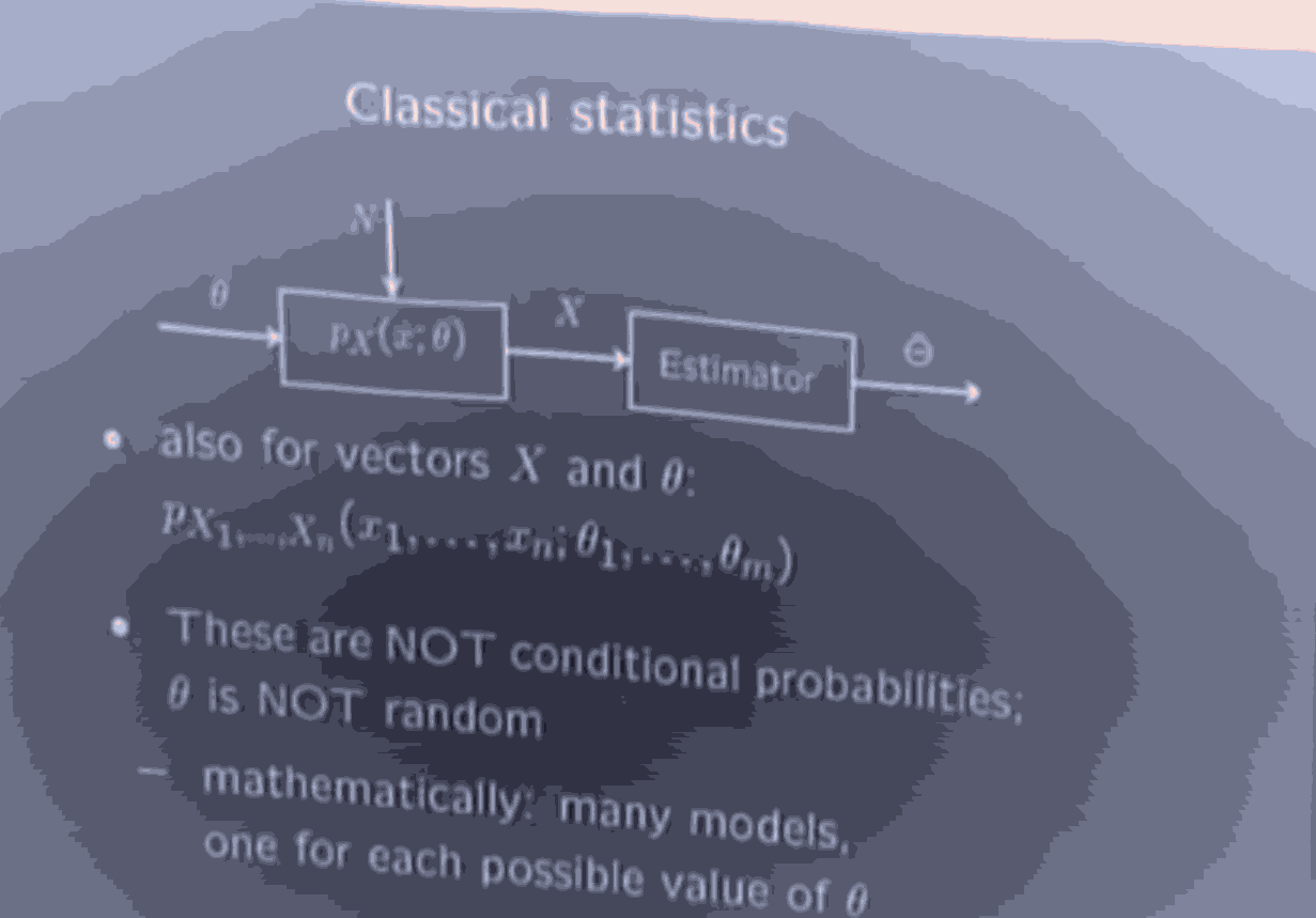
Classical inference

Basically, here, we dont treat the input as a random variable. Rather, we might think about the input as a collection of parameters, that models our noisy measurements $p_X(x;\theta )$.
That is, we have different models or distributions on our measurement $X$, and all of these together are parametrized by values of $\theta$.

So how do we get a good estimator then? We use maximum likelihood. That is, for an estimation problem, in the classical setting, we simply want to pick ${\theta }^{\ast }=\arg \underset{\theta }{max}{p}_X(x;\theta )$. if we make a single measurement, we want to pick the parameters that make this measurement most probable. if we make a vector of measurements, (x is a vector) then we want the parameters that make this vector of measurements as highly probably as we can.

Compare this with beysian map inference, ${\theta }_{map}=\arg \underset{\theta }{max}{p}_{\mathrm{\Theta }|X}(\theta |x)$. using bayes rule, ${\theta }_{map}=\arg \underset{\theta }{max}\frac{p_{X|\mathrm{\Theta }}(x|\theta )p_{\mathrm{\Theta }}(\theta )}{p_X(x)}$. Now, the denominator doesn't contain theta, and moreover, if we assume an "uninformative prior" where every $\theta$ is equally likely, then $p_{\mathrm{\Theta }}(\theta )$ is a constant, so under these conditions,
${\theta }_{map}=\arg \underset{\theta }{max}{p}_{X|\mathrm{\Theta }}(x|\theta )$. Since the distribution on $\mathrm{\Theta }$ is uniform, there must be some probability model $q_X(x;\theta )$ parametrized by $\theta$ giving probabilities that $X=x$. Why is it so? well because the distribution of $\mathrm{\Theta }$ is already fixed, and decided to be uniform, so two different ${\theta }_1,{\theta }_2$ are equally likely. so we can say that each ${\theta }_i$ specifies a probability distribution on $X$, that has nothing to do with how likely ${\theta }_i$ is, because all of them are equally likely.

Hence, in the case of an uninformative (uniform) prior distribution, Map inference and MLE (maximum likelihood estimation) are equivalent.

So we can write ${\theta }_{ML}=\arg \underset{\theta }{max}{p}_X(x|\theta )$. in particular, if $X$ models a vector of independent observations, ( a joint distribution of $X_1,X_2,...X_n$) Then,
${\theta }_{ML}=\arg \underset{\theta }{max}\prod _{i=1}^n{p}_{X_i}(x_i|\theta )$
Let us say we want to find the derivative of $T=\prod _{i=1}^n{p}_{X_i}(x_i|\theta )$, wrt to $\theta$ then due to the chain rule of multiplication, we need to take the derivative of $p_{X_i}(x_i|\theta )$, and multiply with with all other terms in the product: do this for each $i=1\to n$, and add them all up. So we are doing about $O(n^2)$ multiplications and additions.
since $x\mapsto -\log (x)$ is strictly decreasing, equivalently, instead of maximzing $p_X(x|\theta )$ we can minimize $Q=-\log (p_X(x|\theta ))$, whose derivative wrt to $\theta$ is much easier to calculate. Thati is, $$ \theta_{ML} = \arg \min {\theta} \sum^n -\log(p_{X_{i}}(x_{i}|\theta))$$

And $$\frac{dQ}{d\theta} = \sum_{i=1}^n \left(\left(\frac{{d}}{d\theta}{p_{X_{i}}(x_{i}|\theta)}\right) \cdot \frac{1}{p_{X_{i}}(x_{i}|\theta)}\right)$$ where only requires a linear number of terms.

The negative log probabilities, are also tied to information theory. Where the entropy of the random variable, is the expectation of the random variable obtained by taking negative log on the original one. $H[X]=E[-\log (X)]$.

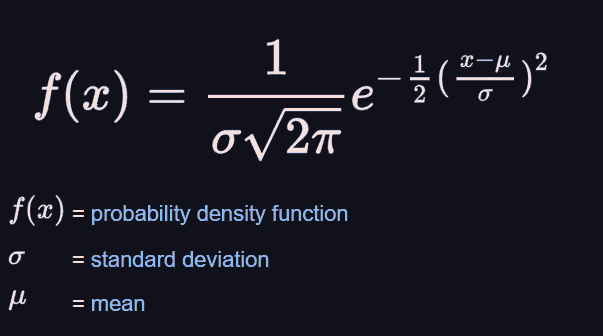
So now an interested problem. Suppose we draw $x_1,x_2,\dots x_n$ from a gaussian distribution with variance $1$. what is the MLE of the mean?

So thats a gaussian. but if the variance is $1$, then $\sigma =1$ as well. so $$f(x) = ce^{-{(x-u)^2}/2}$$

So $X$ is the random variable resenting the joint, independent variables $X_1,X_2,...X_n$, each $X_i$ has the same gaussian $f(x)$ on it as a distribution. so we want to calculate the probability of getting $x=x_1,x_2,..,x_n$
so $$p_X(x|\mu) = \prod_{i=1}^np_{X_{i}}(x_{i}) = c^n\prod_{i=1}^ne^{-{(x_{i}-\mu)^2/2}}$$
Hence it is sufficient to maximize $$T(\mu) = \prod_{i=1}^ne^{-(x_{i}-\mu)^2/2}$$
Equivalently we can minimize (by taking -log on both sides) $$ Q(\mu) = \sum_{i=1}^n(x_{i}-\mu)^2 = \sum_{i=1}^nx_{i}^2 +n\mu^2 - 2\mu\sum_{i=1}^nx_{i}$$ Doing some calculus, and moving things around, we find the obvious $$ \mu_{ML} = \frac{\sum_{i=1}^nx_{i}}{n}$$

We can say that this ${\mu }_{ML}$ is actually a random variable that depends on the random variables $X_1,X_2,\dots X_n$ (which in our case is the same random $X$ variable sampled over and over).

So this is a random variable that depicts the estimator of the true mean $\mu$. What is the expected value of this random variable? That is on average, when we do this sampling process many times and get many different ${\mu }_{ML}$'s, what would be the average $u_{ML}$ we see?

well since in this case, each $X_i$ has the same gaussian distribution with mean $\mu$, it turns out that the average $u_{ML}$ is actually the correct mean $\mu$ which we are trying to estimate.

In other words, the random variable MLE estimator of $\mu$, ${\mathrm{{\rm Y}}}_{ML}$ is expected to be the true mean $\mu$ itself. This means that our estimator is unbiased. On average, it does not favour something larger or smaller than the unknown it's trying to estimate.

So then, We might consider an estimator that we get by applying MLE to some noisy measurement $X$ who distribution is parametrized by the unknown $\theta$ we want to estimate.
call this estimator random variable ${\hat{\mathrm{\Theta }}}_n(x;\theta )$ Where this estimator depends on the vector $x=x_1,x_2,\dots x_n$ we independently sampled (each from $X$ which comes with a model of our noisy measurements) when the true input parameter was $\theta$.

Then, it is nice if the following properties hold for all $\theta$:

• Unbiased : $E[\widehat{{\mathrm{\Theta }}_n}]=\theta$. Now this is sometimes hard to come by for MLE estimators in general, but there are some nice asymptotic properties, for example that as we increase $n$ (the number of measurements we make) The estimators become more and more unbiased.
• Consistency $\widehat{{\mathrm{\Theta }}_n}⟶\theta$. That is, under probability measure (which is also a probability metric), Our estimator converges to the true parameters.