6 - Probability - Continuous RV

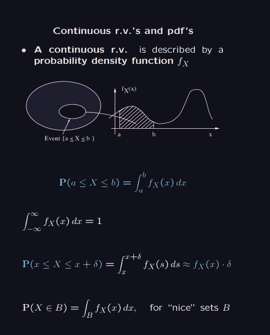
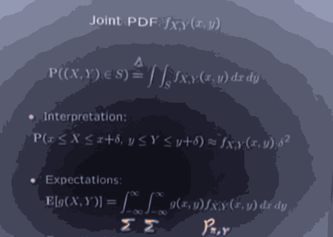
We can use the same ideas, and do the syntactic analogies from sums to integrals.

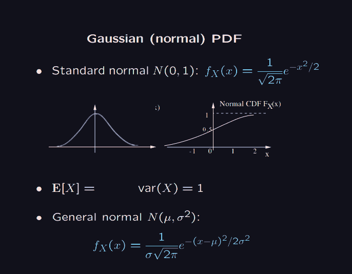
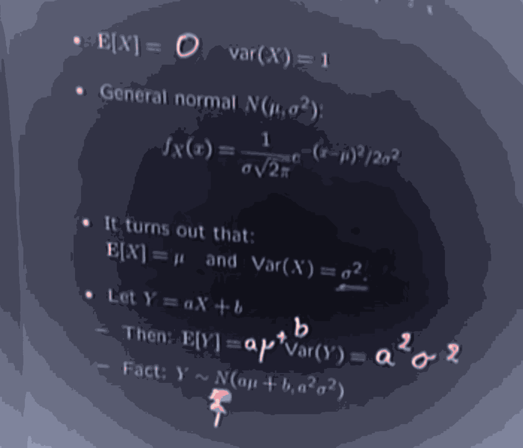
Here, the $f_X$ are called probability density functions.
We have for example the uniform distribution, which looks like $f_X(x)=\frac{1}{b-a}\text{if}a\le x\le b\text{else}0$.
In this case $E[X]={\int }_a^b\frac{x}{b-a}dx=\frac{b+a}{2}$. Which is what we expect, if everything is uniform, we are likely to pick the middle value. and ${\sigma }_X^2=\frac{(b-a{)}^2}{12}$.


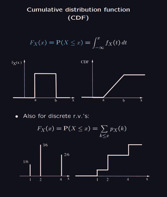
So the cumulative distribution function, at $x$ is the probability that the random variable $X$ outputs something at most $x$. This is nice because they give some unified way of reasoning with both discrete and continuous random variables.






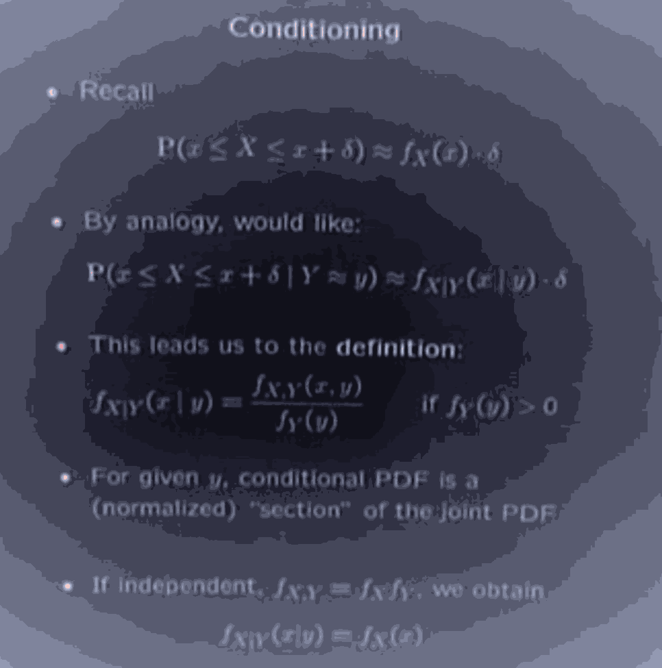
Let us dive deeper into bayes and conditioning.
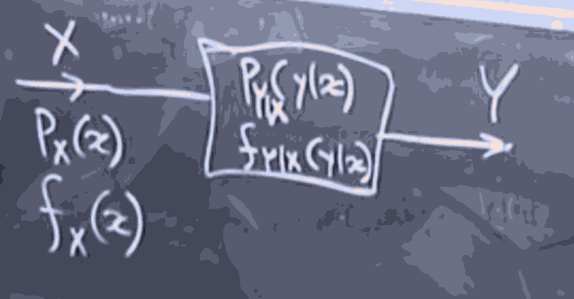
Suppose we have a random variable $X$, and we know it's distribution $p_X(x)$ when discrete (pmf) or $f_X(x)$ when continuous (pdf). So the idea is that we know the DISTRIBUTION of $X$, which goes through some blackbox that is kind noisy, and we get a random variable $Y$, the thing is, we can observe the values of $Y$ only. Our model for the blackbox is the distribution $Y|X$, that is what is the probability (mass or density) of observing any $y$ given some $x$
Now, what is the inference problem here?
Observing some $y\in Y$ collapses the real world into a state where we have observed this $y$. Given this observation, what was the likely state of $X$? that is, we want to model the distribution $X|Y$.
having observed some $y$, we want to know the probability that any $x$ went into the blackbox.

In another way, having observed $Y$, we want to make inferences about $X$.

In particular, if we observe some $x$ and then some $y$, then it is same as observing the pair $(x,y)$, which is the same as observing some $y$ and then some $x$.

allowing $h$ to denote either probability mass or density (depending on discrete/continous)
$h_X(x)h_{Y|X}(y|x)=h_{X,Y}(x,y)=h_Y(y)h_{X|Y}(x|y)$

Hence $h_{X|Y}(x|y)=\frac{h_X(x)h_{Y|X}(y|x)}{h_Y(y)}$ (the bayes rule)
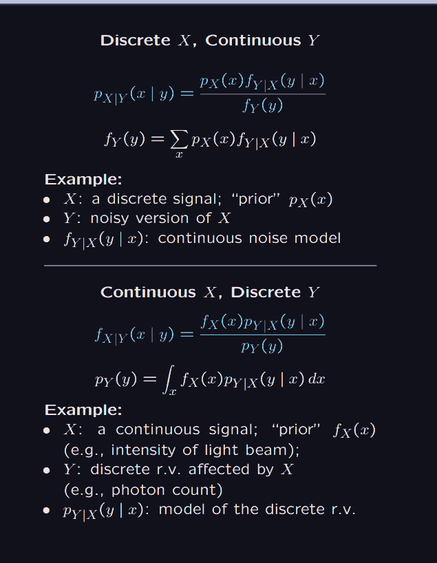
for example let us say $X$ is a signal, and we know its distribution $f_X(x)$ (often called "prior"), and it goes through some noisy blackbox, which gives us an observable random variable $Y$, moreover, let us say we have a model of the noise $f_{Y|X}(y|x)$.

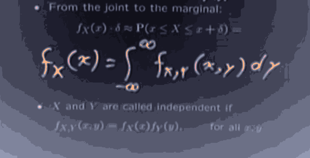
From this information, we can calculate the marginal distribution $h_Y(y)={\int }_{x}h(x)h_{Y|X}(y|x)dx$.
And then using the bayes rule, we can infer the distribution $h_{X|Y}(x|y)$.