5 - Probability - Discrete RV

Sample space, probability measure

The set of all possible outcomes of an experiment, such that exactly one of them occurs whenever we do the experiment, (mutually exclusive outcomes and exhaustive space of outcomes) like for example the outcome of a coin toss can't be both "H" and "T". Sample spaces are usually denoted $Ω$ .
Certain subsets of $Ω$ are called "measurable", and for all such subsets, we can assign a probability measure to them, so if $Σ$ is the collection of measurable subsets, then probability measure is a function $p : Σ \to [0, 1]$ . $Σ$ is called a sigma algebra on $Ω$ and is stable under countable union, compliment, and countable intersection, moreover $Ω \in Σ$ .
There are three axioms on $p$ :
$p (Ω) = 1$
$p (A) \geq 0$
if $A \cap B = ϕ$ , $p (A \cup B) = p (A) + p (B)$ .
if $Ω$ is discrete and finite, the uniform probability measure of $A \subset Ω$ is $| A | / | Ω |$ .
if $Ω$ is continuous, then the uniform probability measure is the "area or nd-volume"
Note: Zero probability does not mean impossible. Points in continuous spaces have zero probability, yet the outcome of a certain experiment can be a single point. Similarly probability 1 does not mean the event occurs all the time. for example, the probability of getting any point on the uniform unit square, that isn't the origin is 1. (the origin has zero probability) yet ofc we can pick the origin.

Support/Figures/Pasted image 20250115020236.png

conditional probability

If we get some partial information that event $B$ has occurred, Then the probability that event $A$ occurs given $B$ is : $p (A | B) = \frac{p (A \cap B)}{p (B)}$ . This is essentially shifting the universe to $B$ . The axioms of probability measure still holds in this universe. for example, $p (A \cup B | C) = p (A | C) + p (B | C)$ as long as $A, B$ are disjoint.
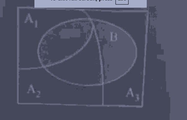
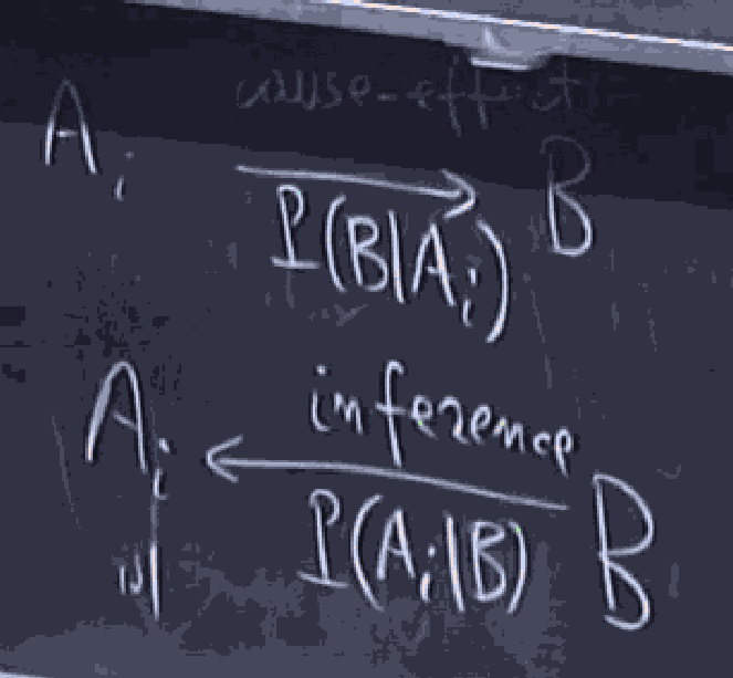
Suppose we partition $Ω$ into events $A_{1}, A_{2}, . ., A_{m}$ . And $B$ is also an event. Then, $p (B) = \sum_{i = 1}^{m} p (B \cap A_{i}) = \sum_{i = 1}^{m} p (A_{i}) p (B | A_{i})$
if we want to calculate $p (A_{j} | B) = \frac{p (A_{j} \cap B)}{p (B)}$ , then we can write $p (A_{j} \cap B) = p (B \cap A_{j}) = p (B | A_{j}) p (A_{j})$ .
Hence, $p (A_{j} | B) = \frac{p (B | A_{j}) p (A_{j})}{\sum_{i = 1}^{m} p (A_{i}) p (B | A_{i})}$ .
This is known as the baye's rule.
An alternative statement with $m = 1$ , is $p (A | B) = \frac{p (B | A) p (A)}{p (B)}$ .
Support/Figures/Pasted image 20250115021451.png

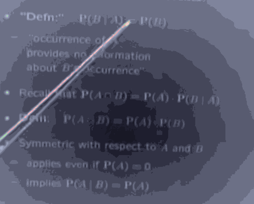
If the occurrence of event $A$ produces no information about the occurrence of event $B$ (and vice versa), these events are independent.
Support/Figures/Pasted image 20250115022017.png
In a conditional universe, if given the occurence of $C$ , the occurence of $A$ produces no information about the accurence of $B$ , then $p (A \cap B | C) = p (A | C) p (B | C)$ (this is called conditional independence).

If we had a game, where $Ω$ is some set of events, and $X : Ω \to R +$ is the payoff of each event. with the payoff of $x$ dollars occurring with probability $p_{X} (x)$ . What is the expected payoff of this game?
If we play this game $N$ times, we are paid, $x$ dollars roughly $p_{X} (x) * N$ times, for each payout $x$ . As $N$ gets very large, for each $i = 1$ to $n$ , we are paid $x_{i}$ amount about $p_{X} (x_{i}) * N$ times. so in $N$ games, if $N$ is very large, our total payout is $\sum_{i = 1}^{n} p_{X} (x_{i}) * x_{i} * N$ , so averaging it out, the expected value $E (X) = \sum_{i = 1}^{n} p_{X} (x_{i}) x_{i}$ .

Support/Figures/Pasted image 20250115024528.png
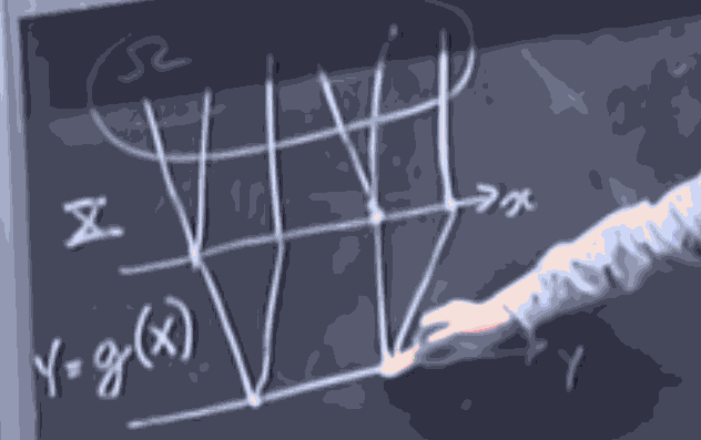
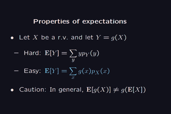
Now, imagine that whenever event $ω \in Ω$ occurs, instead of getting a payout of $X (ω)$ , we get a payout of $g (X (ω))$ This is completely fine! To calculate the expectation of the new random variable $g (X)$ , we know that whenever $(X = x_{i})$ , the payout is instead $g (x_{i})$ .
Hence Allowing $Y = g (X)$ , we have the following picture
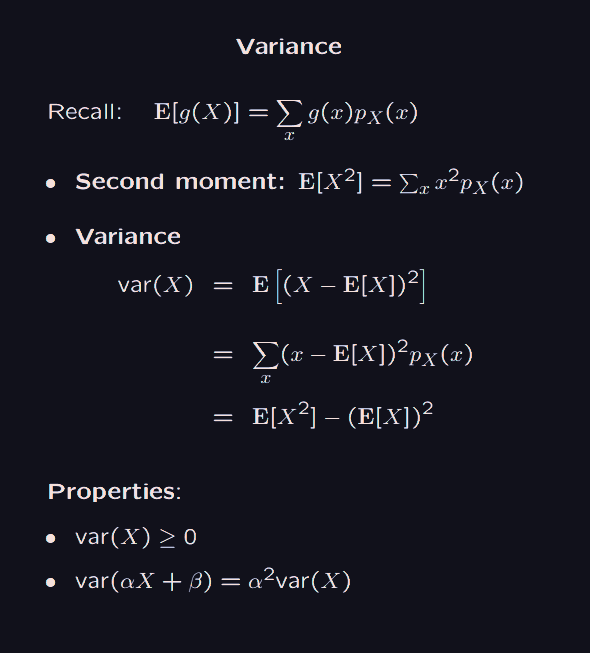
Support/Figures/Pasted image 20250115025153.png

The variance tells you, what is the expected distance of a random variable form it's mean/expected value?, The standard deviation is the square root of the variance.

The conditional expectation of a random variable $X$ given an event $A$ , the sorta the average value we measure of $X$ , given event $A$ has already occurred. again, if $A$ has already occurred, then the probability that we get a payout of $x$ is equal to $p_{X | A} (x)$ , where $p_{X | A}$ is the new probability mass from $X$ to $[0, 1]$ where $p_{X | A} (x) = p ({w \in Ω : X (w) = x} | A)$ .
Hence $E [X | A] := \sum_{x} x p_{X | A} (x)$ .

Imagine partitioning the sample space into $A, A^{c}$ .
for any $x$ being the output of the random variable $X$ ,
we have that $p_{X} (x) = p (A) p_{X | A} (x) + p (A^{c}) p_{X | A^{c}} (x)$
This is because in a mutually exclusive manner, either event $A$ occurs, and we enter the context where the probability mass of $X$ is conditioned on $A$ , or $A^{c}$ occurs, entering the probability mass of $X$ conditioned on $A^{c}$ . Hence, we can write that $E [X] = p (A) E [X | A] + p (A^{c}) E [X | A^{c}]$
In general, $$E(X) = \sum_{i=1}^np(A_{i})E[X|A_{i}]$$ where $A_{1}, \dots A_{n}$ is a partition of the sample space.

let $X$ be a random variable indicating the number of independent coin tosses after which we see the first "Heads".
Here the space of events is any sequence of $n$ coin flips, for any $n \in N$ .
Now, we can partition this space into two events.
let $A$ be the set of all events where the first flip was a tail. and $A^{c}$ be the set of all events where the first flip was a head.
Then $E [X] = p (A) E [X | A] + p (A^{c}) E [X | A^{c}]$
But $A^{c}$ is the set of all events where the first flip is "Heads", therefore, $E [X | A^{c}] = 1$ . But $A$ is the set of all events where we flip a tail on the first flip. Since we have already flipped a tail, and subsequent coin tosses are independent, we have effectively come back to the same probability mass on $X$ , but we have spent one extra flip. Hence $E [X | A^{c}] = E [X + 1]$ , using linearity of expectation, we get $E [X] = (1 - p) (E [X] + 1) + p$ . Hence $E [X] = 1 / p$ .

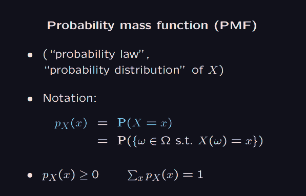
Joint distributions:

if $X, Y$ are random variables, with mass functions $p_{X}, p_{Y}$ , the joint distribution $p_{X, Y} (x, y) := P (X = x and Y = y)$ . We still have that $\sum_{y} \sum_{x} p_{X, Y} (x, y) = 1$
To extract the probability mass $p_{X}$ , we have $p_{X} = \sum_{y} p_{X, Y} (x, y)$ . This is called the marginal distribution of $X$ , where we are marginalizing out $Y$ .

Now, the joint conditional distribution $p_{X | Y} (x | y) := P (X = x | Y = y) = \frac{p_{X, Y} (x, y)}{p_{Y} (y)}$ . Here, we imagine fixing an output of the random variable $Y$ as $y$ and for each such fixture, $p_{X | Y} (x | y)$ has the same "shape" as the "slice" of the joint distribution at that particular $y$ , but is re-scaled by the marginal of $Y$ at that $y$ , to ensure that the probabilities add up to 1.

Just generalizing, suppose $< X_{i} >$ is a list of random variables, which take on tuple values $< x_{i} >$ for $i = 1 \to n$ .

using our intuition, if $< X_{i} >$ takes values $< x_{i} >$
Then first $X_{1}$ takes value $x_{1}$ , then conditioned to that, $X_{2}$ takes value $x_{2}$ , then conditioned to both of those, $X_{3}$ takes value $x_{3}$ and so on.

Hence $$p_{X_{1},X_{2},\dots X_{n}}(x_{1},x_{2},\dots x_{n}) = \prod_{i=1}^n p_{X_{i}|X_{1}, X_{2}, \dots X_{i-1}}(x_{i}|x_{1},x_{2},\dots x_{i-1})$$
Where the $i t h$ variable is condition on all the previous ones.
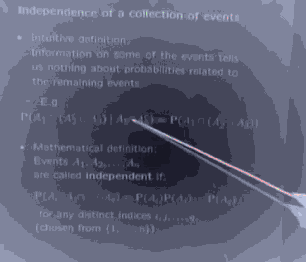
Now, if it is true that these $n$ random variables are pairwise, triple-wise and so on independent, that is the occurrence of any sub-set of these random variables taking some value, gives no information about any other random variable, then for any sub-set indexer $a_{1}, \dots a_{k}$

p_{X_{a_{1}} | X_{a_{2}, \dots X_{a_{k}}}} (x_{a_{1}} | x_{a_{2}}, \dots x_{a_{k}}) = P_{X_{a_{1}}} (x_{a_{1}})

So if $n$ random variables are independent, then using the conditional expression seen above, with the other expression even more above, we get:

p_{X_{1}, X_{2}, \dots, X_{n}} (x_{1}, x_{2}, \dots x_{n}) = \prod_{i = 1}^{n} p_{X_{i}} (x_{i})

That is, if the random variables $X_{1}, X_{2}, \dots X_{n}$ are independent, their joint probability mass is the product of each marginal probability mass.

If $X_{1}, X_{2}, . . X_{n}$ are random variables, with the tuple $(x_{1}, x_{2}, \dots x_{n})$ giving $g (x_{1}, x_{2}, \dots x_{n})$ payout, then the expected value: $$E[g(X_{1},X_{2},\dots,X_{n})] = \sum_{x_{1}\in X_{1}} \sum_{x_{2} \in X_{2}} \dots \sum {x \in X_{n}} g(x_{1},x_{2},\dots x_{n}) p_{X_{1},X_{2},\dots X_{n}}(x_{1},x_{2},\dots, x_{n}) $$

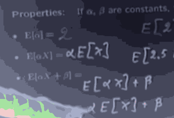
Here again, we can show linearity, let $g$ be the map $(x_{1}, x_{2}, \dots x_{n}) \mapsto a_{1} x_{1} + a_{2} x_{2} + \dots a_{n} x_{n}$ Just using our eyes and mind and the distributive law, and factoring things out, we have:

E [\sum_{j = 1}^{n} a_{j} X_{j}] = \sum_{j = 1}^{n} a_{j} E [X_{j}]

So the expectation of a linear combination of random variables, is the linear combination of the expectation of random variables :)

now if $g$ is the product function $(x_{1}, x_{2}, \dots x_{n}) \mapsto \prod_{i = 1}^{n} x_{i}$ , moreover if the $n$ random variables are independent, then:

E [\prod_{j = 1}^{n} X_{j}] = \sum_{x_{1} \in X_{1}} \dots \sum_{x_{n} \in X_{n}} (\prod_{j = 1}^{n} x_{j} P_{X_{j}} (x_{j}))

in the innermost product, the first $n - 1$ terms are independent of the last summation which sums over only possible values of the random variable $X_{n}$ hence, we can factor them out:

E [\prod_{j = 1}^{n} X_{j}] = \sum_{x_{1} \in X_{1}} \dots \sum_{x_{n - 1} \in X_{n - 1}} (\prod_{j = 1}^{n - 1} x_{j} P_{X_{j}} (x_{j}) \sum_{x_{n} \in X_{n}} p_{X_{n}} (x_{n}))

equivalently

E [\prod_{j = 1}^{n} X_{j}] = \sum_{x_{1} \in X_{1}} \dots \sum_{x_{n - 1} \in X_{n - 1}} (\prod_{j = 1}^{n - 1} x_{j} P_{X_{j}} (x_{j}) E [X_{n}])

Continuing this process, we get

E [\prod_{j = 1}^{n} X_{j}] = \prod_{j = 1}^{n} E [X_{j}] $ $ W h e n e v e r t h e $ n $ r a n d o m v a r i a b l e s a r e i n d e p e n d e n t . M o r e o v e r, i f $ X_{1}, X_{2}, . ., X_{n} $ a r e i n d e p e n d e n t, t h e n $ g_{1} (X_{1}), g_{2} (X_{2}), \dots g_{n} (X_{n}) $ a r e a l s o i n d e p e n d e n t . I m e a n n o m a t t e r w h a t v a l u e $ X_{j} $ t a k e s, i t g i v e s m e n o n e w i n f o r m a t i o n a b o u t $ X_{k} $, h e n c e I g e t n o n e w i n f o r m a t i o n a b o u t $ g_{k} (X_{k}) $, t h e r e f o r e $ g_{j} (X_{j}) $ c a n n o t g i v e n e w i n f o r m a t i o n a b o u t $ g_{k} (X_{k}) $ e i t h e r (t h i s i s a v e r y i n f o r m a l v i e w, w e w i l l g e t t o i n f o r m a t i o n t h e o r y l a t e r) H e n c e, $ $ E [\prod_{j = 1}^{n} g_{j} (X_{i})] = \prod_{j = 1}^{n} E [g_{j} (X_{i})]

Notice that for variance, $var (X + Y) = E [(X + Y - E [X + Y])^{2}] = E [(X + Y)^{2}] - (E [X + Y])^{2}$ Solving, we get

var (X + Y) = E [X^{2}] + E [Y^{2}] + 2 E [X Y] - (E [X]^{2} + E [Y]^{2} + 2 E [X] E [Y])

Now, if $X, Y$ are independent, $E [X] E [Y] = E [X Y]$ Therefore,

var (X + Y) = E [X^{2}] - E [X]^{2} + E [Y^{2}] - E [Y] = var (X) + var (Y)

Indeed by induction if $X_{i}$ for $i = 1 \to n$ are all independent of each other, $var (\sum_{i = 1}^{n} X_{i}) = \sum_{i = 1}^{n} var (X_{i})$ .

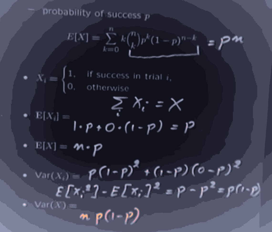
Binomial distribution, is the random variable X, which counts the number of successful trails of $n$ independent trials, where the probability of success is $p$ , and failure is $(1 - p)$ . We can use the indicator variable trick.
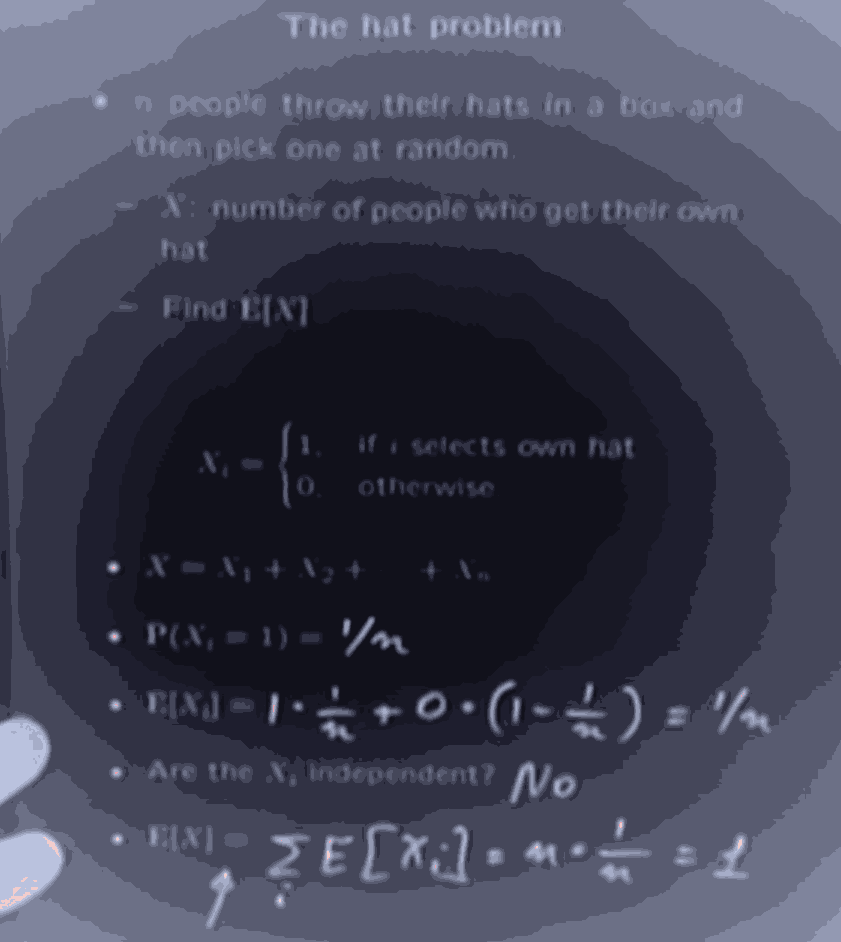
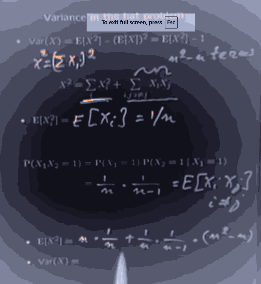
Support/Figures/Pasted image 20250115222017.png
The good thing about expected value is that it doesn't care about independence.

in the above problem, the $X_{i}$ $i = 1 \to n$ are not independent. if I tell you that each $X_{i}$ from $i = 1 \to n - 1$ are all 1, that means that the last remaining hat is the hat of the $n t h$ person, so it does change the probability of the nth guy finding his hat, from 1/n given no information to 1 giving this peice of information.
Support/Figures/Pasted image 20250115222735.png