1 - Attention is all you need - Training

note, we will adopt a row first approach as is the nature of pytorch, even though column vectors as features agree with linear algebra convention more.
Now, there is a lot of oversimplification as to how a transformer actually works. Let us start with a very simple idea.
let us say we have an input sequence $s 1, s 2, s 3$ and a target sequence $t_{1}, t_{2}, t_{3}, t_{4}$ .
During training(for autoregressive models): $s 1 = t 1, s 2 = t 2, s 3 = t 3$ and we want to predict $\hat{T} = \hat{t_{1}}, {\hat{t}}_{2}, {\hat{t}}_{3}, {\hat{t}}_{4}$
Actually what happens is: we pass $S = [s_{1} s_{2} s_{3}]$ as a matrix to the "encoder block" and we right shift the target $T = [< s > t_{1} t_{2} t_{3}]$ into the "decoder block".
So given $S, T$ we need to produce a $\hat{T}$ .
And the loss is then $\hat{T}$ against $t_{1}, t_{2}, t_{3}, t_{4}$ .

So to be very clear, in order to predict a 4 length sequence from a 3 length sequence, we need to pass the 3 length sequence into the "encoder block", Pass a right shifted target sequence (which is the same as the input sequence if its an autoregressive task, or its different for translation type stuff). And then using both, we predict the entire output sequence and evaluate it against the full target sequence (both of length 4).
Support/Figures/Pasted image 20250519172942.png

So, let $S = s_{1}, s_{2}, . . . s_{T}$ and $T = t_{1}, t_{2}, t_{3} . . t_{T + 1}$ both as matrix-one-hots.

then, we pass $S$ into the "encoder" and $T_{s h i f t} =< s >, t_{1}, t_{2}, \dots t_{T}$ into the "decoder". In theory, the prediction is auto-regressive, in the sense that only $< s >, s_{1}$ is used to predict $t_{1}$ , (where $t_{1} = s_{1}$ in auto-regressive non translation type stuff).
and so on. In practise, $S, T_{s h i f t}$ are passed at once, and we use attention and masking to parallel emulate auto-regression.

we predict $\hat{T} = {\hat{t}}_{1}, \dots {\hat{t}}_{T + 1}$ and then take $L o s s (T, \hat{T})$ .

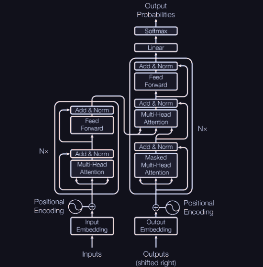
Let us see what's happening at a high level here:
first $E S = e m b (S)$ we embed the one hot vectors into some vector space.

Then we introduce some positional encoding $X = P o s (E S)$ . Then we feed it through $N_{l a y e r}$ encoder blocks $H = e n c^{N_{l}} (X)$ notice that each encoder layer is different, and power is used to denote applying them sequentially because I like brevity.

So $H$ is the encoding. Now there are $N_{l a y e r}$ decoder blocks as well. And each decoder block recives $H$ in its forward pass! Moreover the first decoder block receives $Y^{*} = p o s (E T_{s h i f t e d})$ where $E T_{s h i f t e d} = d e c o d e r_{e m b} (T_{s h i f t e d})$ and $p o s$ is as usual a positional encoding.
$G = d e c^{N_{l a y e r}} (H, Y^{*})$
then $\hat{T} = s o f t m a x (l i n e a r (G))$ , and loss is $c r o s s E N T (\hat{T}, T)$ .

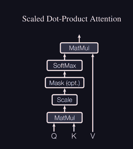
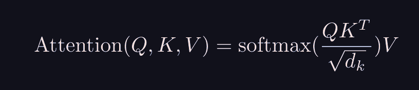
Self-Attention: Scaled-Dotproduct:

so, given an embedding matrix $X$ of shape $(T, d_{m o d e l})$ we make three linear projections of this model: $K = X W_{k}$ $Q = X W_{Q}$ $V = X W_{V}$ .
both $W_{K}, W_{Q} \in R^{d_{m o d e l} \times d_{k}}$ or $(d_{m o d e l}, d_{k})$ $d_{k}$ is the key/query dimension. and $W_{V}$ has shape $(d_{m o d e l}, d_{v})$

Support/Figures/Pasted image 20250519182016.png

Support/Figures/Pasted image 20250519182042.png

So we compute the dot product between the $Q$ and $K$ matrices, and then scale it by the key dimension. we also optionally mask the upper-triangle with -inf to zero out the attention of future time-steps with current ones. and then finally matmul by $V$ .

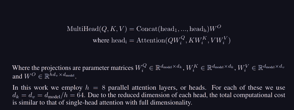
it is pretty clear that the output of a single attention head has shape $(T, d_{v})$ . as the $Q K^{T}$ has shape $(T, T)$ computing the attention pattern. Support/Figures/Pasted image 20250519182620.png

For multi head attention, we use the same embedding matrix and pass it through different heads. we choose $d_{v}$ to be $d_{m o d e l} / h$ so that after concatenating the outputs of multiple heads and matmul by $W^{O}$ we get a matrix of shape $H_{o u t} = (T, d_{m o d e l})$ again. Once we understand attention, there is not much else to the architecture:

Encoder block:

does multi head attention and a residual connection adds the original embedding to the output of the multi head attention. Then we normalize, then pass through an MLP and then do another residual connection and normalize again

L = n o r m (M H_{a t t n} (X) + X)

e n c = n o r m (M L P (L) + L)

so applying multiple encoder layers in chain gives us the final encoding $H$ . For an encoder block which isn't the first one, we use the output of the previous encoder block in place of $X$ .

Decoder block:

once encoding is done, let $Y *$ be the position-ally encoded, embedded version of $T_{s h i f t e d}$ .
Then, for the first decoder block,

A = n o r m (M a s k e d M u l t i H e a d_{a t t n} (Y^{*}) + Y^{*})

B = n o r m (M u l t i H e a d_{a t t n} (H, A) + A)

C = n o r m (M L P (B) + B)

and for future decoder blocks, the previous block's output is used in place of $Y^{*}$ and the encoded matrix $H$ is passed to EACH DECODER LAYER.

finally we apply multiple decoder layers and then a linear followed by softmax to get $\hat{T}$ , and do grad descent on cross entropy between $\hat{T}$ and $T$ .

A small caveat,in actuality,the encoder-decoder attention, the one that we wrote $B = n o r m (M u l t i H e a d_{a t t n} (H, A) + A)$ actually uses the final stored $K, V$ matrices from the final encoder head (from the output encoder head) and the $Q$ comes from the previous decoder layer.
For all other attention heads, it uses its own $K, Q, V$ as usual.

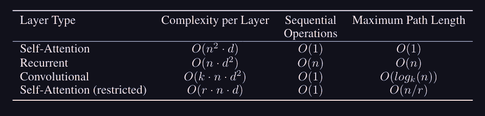
Why attention?

Support/Figures/Pasted image 20250519185144.png
so here, (in self attention) per layer, we only do 1 sequential operation, the complexity per layer is fully parallelised. Moreover, the most important thing is that the number of forward props we need to do to process a full sequence is just one. (upto big O). In a recurrent model, if the seq length is $n$ we need to do $n$ forward props and then BPTT. but transformers process sequences in one batched go. so the forward prop path length is constant, independent of sequence length in a transformer.

Superposition:

In theory we would love for each semantic "idea" to be embedded into perpendicular dimensions. That is if d_model = N, then we can encode $N$ different semantic ideas as perpendicular directions, and represent a combination of ideas as component sums of each direction.
However, if one relaxes and allows an $ϵ$ free perpendicular encoding of semantics, that is each semantic is at most $ϵ$ angle away from being perpendicular to any other semantic, then the number of directions grows as $e^{(ϵ N)}$ !!!! So in this case, we have exponential growth in the number of possible directions for a "semantic feature", however this also means that most semantic features are not a single direction or a single neuron, which is one of the theories on why LLM interpret-ability is hard.

We will reserve implementation and training details to another time, this was just the core architecture.

Sources: 3b1b deep learning series, Attention is all you need paper, my brain.