Hyperparameter Tuning - 1

In essence, the neural network we initialize doesn't have to depend on the number of training examples. The weight and bias matrices that we initialize before hand only depend on the vector dimensions of the layers.
It is therefore possible to have different number of training examples, on the train, development (validation), and test data sets, and the number of training examples can be extracted during the forward propagation step.

def init_NN (HL_dims (list), A0_dims, AL_dims): 
	layer_dims = [A0_dims] + HL_dims + [AL_dims]
	n = len(layer_dims)
	weight_array = [radom__matrix(layer_dims[i+1],layer_dims[i]) for i in [0,n-1)]
	bias_array = [zeros(layer_dims[i+1]) for i in [0,n-1)]
	dW_array = [zeros(layer_dims[i+1],layer_dims[i]) for i in [0,n-1)]
	db_array = [zeros(layer_dims[i+1]) for i in [0,n-1)]
	
	
def forward_propogation(nerual_network, X):
	m = X.shape[1]
	'''
	A_array, dA_array, Z_array, dZ_array = [zeros(layer_dims[i], m) for i in [0,n-1)]
	#Do_forward_Prop_On_X
	
	'''

As a rule of thumb, with smaller data, let say 1000 examples, we might do 70/15/15 split for the train, dev, test sets, or 60/20/20
but with larger data, say 1,000,000 examples, we might do just 10,000 examples for dev and test septs, which would be a 98/1/1 split.
Moreover it is important to have our train, dev, test sets all from the same distribution, let's say our cat/non-cat pics are from google for the train set, but the dev and test sets are taken from the phone, this might not be a good idea :)

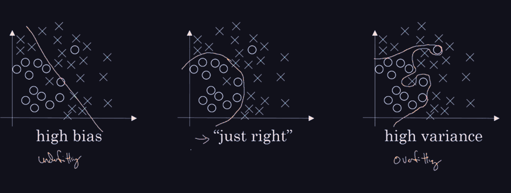
Bias, Variance

Support/Figures/Pasted image 20240914081148.png
if we can't even fit well on the train set, let's say train set error is 20%, that might be a high bias (underfit case)

if we do very well on the training set, let's say train set error is 1% but dev set error is 10%, then, we have an overfit on the train set.
It's possible to have both high-variance and high-bias.

if the Bias is large, we want to fit better on the train set:
Try: more iterations, lower learning rate, get a bigger network (more layers) and all that good stuff.

if the bias is now small, but the variance is large, we can always get more data, use regularization and so forth.

Solving Overfitting Via Regularization:

Let $\hat{Y}$ be the output of a neural network $F (W^{[1]}, \dots W^{[L]}, B^{[1]}, \dots B^{[L]})$ . The idea of $L 1$ and $L 2$ regularization is that the new cost has an extra term with respect to each weight matrix that needs to be minimized. let $N (W^{[l]})$ be the new norm (either L1 or L2) of the weight matrix at later $l$ , and let $L$ be a loss function, then the new cost is:

\frac{1}{m}\bigg( \sum_{i=1}^m \mathscr L(\hat{Y}^{(i)}, Y^{(i)}) + \sum_{l=1}^{L} \lambda N(W^{[l]})\bigg )$$ where $\lambda$ is the regularization parameter. The rough idea here is that we want to minimize the norm of our weight matrix, in addition to the actual cost, this way, some of our weights will be so small, that they kind of "dampen" the contribution of certain features, helping the model not be "over-reliant" on certain features, or in another sense, the bigger the $\lambda$ the more zeroed out certain weights will be, sorta simplifying and hazing out the complex neural network which otherwise might capture a lot of unnecessary detail. Increasing $\lambda$ will move us from overfitting towards underfitting, but hopefully there's a sweet spot in the middle :) ##### L2 regularization: The $L_2$ norm (Forbenious norm) of a matrix is $$\lvert W \rvert_{F} = \sum_{i}\sum_{j} w_{ij}^2 $$ Hence, the derivative of this matrix is simple $2W$. Hence our new costs might look like: $$ C_{l} =\frac{1}{m}\bigg( \sum_{i=1}^m \mathscr L(\hat{Y}^{(i)}, Y^{(i)}) + \sum_{l=1}^{L}{\frac{\lambda}{2}} |W^{[l]}|_{F}\bigg)

Where $C = \frac{1}{m} (\sum_{i = 1}^{m} L ({\hat{Y}}^{(i)}, Y^{(i)}))$ . And for the update step, allow $d W^{[l]} = \frac{\partial C}{\partial W^{[l]}}$ . Then we have: $$ W^{[l]} \leftarrow W^{[l]} - \alpha\left( dW^{[l]} + \frac{\lambda}{m} W^{[l]} \right)$$

the above process of update is called "weight decay" gradient descent.

Dropout regularization:

let $A^{[l]}$ be the activation matrix of layer $l$ , whose columns are vectors depicting the activations of each training example. we want to crate a mask matrix of the same dimensions a $A^{[l]}$ , call it $D^{[l]}$ to drop out nodes randomly, different for each training example. for every layer, we need a keep-probs scalar $k_{l} \in [0, 1]$ and we will generate a random matrix $D^{[l]}$ and discretize it to ${0, 1}$ using $D^{[l]} < k_{l}$ doing an elementwise truth on the inequality. if $D_{i j}^{[l]} < k_{l}$ ,then we set it to $1$ , and $0$ otherwise. Moreover, we need to scale $A^{[l]}$ down by $k_{l}$ to allow it to have the same expected value as before.
Most definitely, we should only use dropout during the training phase, once all the weights are trained accustomed to the harsh environment of nodes dropping out here and there, we want to freeze the weights in place, and do a normal forward and backward pass on the test and dev sets. Otherwise we would just introduce noise into

So finally, let $A^{' [l]} = f (Z^{[l]})$ where $Z^{l} = W^{[l]} A^{[l - 1]} + B^{[l]}$ . Then $A^{[l]} = \frac{D^{[l]} * A^{'} [l]}{k_{l}}$ .
For the backward propagation, suppose we know $d A^{[l]} = \frac{\partial C}{\partial A^{[l]}}$ . Then, abusing the same notation, $d A^{' [l]} = d A^{[l]} * \frac{D^{[l]}}{k_{l}}$ . And the rest of the backprop stays the same.