Logistic Regression

Suppose we had a collection of $u \times v$ image, that is, it has $u$ rows of pixels, each row containing $v$ pixels. Suppose we want to build a binary classifier model that takes such images, and maps it into two classes { $1$ - cat , $2$ - not cat}.

First, we have to collect the pixel RGB value into a column vector. We do this by reading the image matrix left to right, top to bottom, say R then G then B, and so we have an input vector $x$ of dimension $n_{x} = 3 u v$ .

our training data will be pairs $(x^{i}, y^{i})$ for $1 \leq i \leq m$ . where $y^{i} = 1$ only if $x^{i}$ is a cat, and $y^{i} = 0$ otherwise.
so we will store both $x^{i}$ and $y^{i}$ as columns of matrices. $$X =\begin{bmatrix}
\vdots \ \ \ \ \vdots \ \ \ \dots \ \ \ \ \vdots \
x^1 \ x^2 \ \dots \ x^m \
\vdots \ \ \ \ \vdots \ \ \ \dots \ \ \ \ \vdots \
\end{bmatrix}$$

Notice that each $x^{i}$ is stored as a column vector, and each $y^{i}$ is also (a 1 dimensional) column vector.

Y = [\begin{matrix} y^{1}, y^{2}, \dots, y^{m} \end{matrix}]

A model for binary classification, could take in a weight vector $w$ and maybe do a linear regression ${\hat{y}}^{i} = w^{T} x^{i} + b$ . notice that $w, x \in R^{n_{x}}$ (notice that we will use hat notation to depict model outputs)

But the issue then is, that we want $\hat{y^{i}}$ to somehow capture/approximate the probability that $x^{i}$ is a cat. so we want ${\hat{y}}^{i} = P r (y^{i} = 1 | x^{i})$ . And so we want the output to be bounded in $[0, 1]$ .

Here is where we use the sigmoid function $$\sigma(z) = \frac{1}{1+e^{-z}}$$
Our model is then $$ \hat{y}^i = \sigma(w^Tx^i + b) $$
Now, we need a loss function, $L ({\hat{y}}^{i}, y^{i}) \in R^{+} \cup {0}$ . Such that the following properties hold: $L$ decreases as ${\hat{y}}^{i} - y^{i}$ decreases, and it would be nice if $L$ is convex, as a function of the weights and bias. That way, no matter where we start, our gradient descent will find the global minimum.

We claim that $L = ({\hat{y}}^{i} - y^{i})^{2}$ is not a good choice, because of course $L$ decreases as $\hat{y^{i}}$ gets closer to $y^{i}$ , but $L$ is not convex, as a function of the weights or bias.

It is sufficient to show that $L$ is not convex in the weights, as that would be bad enough. Fix $x^{i}, y^{i}, b$ . then $$ \mathscr L(w) = \bigg({\dfrac{1}{1+e^{-(w^Tx^i + b)}}- y^i}\bigg)^2$$

so if we fix all other weights except $w_{j}$ and parametrize it by $w_{j} = t$ then, $$\mathscr L(t) = \bigg(\frac{1}{1+ e^{-(x^i_{j}t + C)}} - y^i\bigg)^2$$
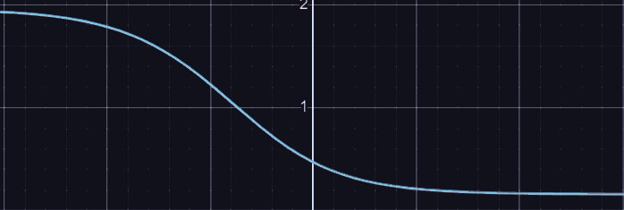
essentially, we have $$\mathscr L(t) =\bigg(\frac{1}{1+ ae^{-bt }} - c\bigg)^2 $$
and we could of course evaluate the second derivative of $L$ , or we could look at the graph. (this for $c = - 1$ ) Support/Figures/Pasted image 20240812193336.png
Notice that the left half is concave, with the function being above the secant line between any two points on the function.

A better loss function:
$L ({\hat{y}}^{i}, y^{i}) = - (y^{i} \log \hat{y^{i}} + (1 - y^{i}) \log (1 - {\hat{y}}^{i}))$
for a fixed $y^{i}$ and $x^{i}$ , it is pretty clear that $L$ depends on the weight vector $w$ , and bias $b$ .
in particular, for ease, let $Δ = w^{T} x^{i} + b$ . and $y^{i} = c$ . Doing some algebra using: $$ \hat{y}^i = \frac{1}{1+ e^{-\Delta}} $$ we get: $$L(\Delta) = \log(e^{\Delta}+1) - c\Delta $$
Finally, we have, that for any weight $w_{j}$ in the weight vector, parametrizing $w_{j} = t$ and fixing all other weights, we have $Δ (t) = t x_{j}^{i} + b + D$ where $D$ is everything in the dot product of $w$ and $x^{i}$ that isn't $w_{j} = t$ times $x_{j}^{i}$ .
Essentially, $Δ (t) = A t + B$ . so $$L(t) = \log(e^{At + B} + 1) - c(At + B)$$
Hence, $$L'(t) = \frac{{Ae^Be^{At}}}{e^{At + B}+1} - cA$$
That is, $$L'(t) = A\bigg(\frac{{e^{At + B}}}{1 + e^{At + B}} - c\bigg)$$

Finally we see that $L$ is convex, with respect to every single weight.

L^{″} (t) = \frac{A^{2} e^{A t + B}}{(1 + e^{- (A t + B)})^{2}} > 0

notice that we had set $w_{j} = t$ to be the moving parameter, and fixed everything else. We could set any weight as the moving parameter $t$ and still obtain $L^{″} (t) > 0$ . Hence, the above inequality essentially says that $\frac{\partial^{2} L}{\partial w_{j}^{2}} > 0$ for each $1 \leq j \leq n_{x}$ . Hence, very informally, no matter in which axis (Imagine the loss function being $L : R^{n_{x}} \to R^{+} \cup {0}$ , being plotted in $R^{n_{x}} + 1$ dimensional space) we perturbate in, the rate of change of the function is increasing. This is especially nice because the whole point of gradient descent to initialize weights as a point $w \in R^{n_{x}}$ then, the following algorithm: $$\text{for} \ j = 1 \ \text{to} \ n_{x} : w_{j} \leftarrow w_{j} - \frac{\alpha {\partial L}}{\partial w_{j}} $$ always finds the (one and only) well because $L$ is strictly convex with respect to each axis/weight $w_{j}$ .
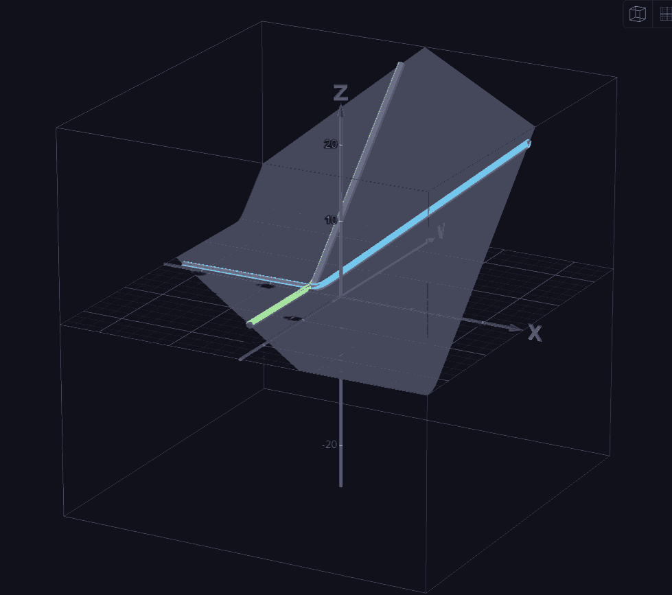
In general, the "well" idea can be seen in the graph of logistic regression with just two weights as the parameters.
![[Support/Figures/Pasted image 20240812223757.png]

here, just think about $x, y$ as weights, and $z$ as the loss function.
Support/Figures/Pasted image 20240812224340.png
if we're restricted to $x > 0, y > 0$ we might start on any large $x, y$ and descend, noticing that as $x$ and $y$ decrease, the slope becomes less and less negative, becoming zero where the red and blue lines cross.

In practice we want to minimize the average loss of the model over the entire training set.
The cost function does this:

J = \sum_{i = 1}^{m} L (\hat{y^{i}}, y^{i})

Indeed, the new algorithm for gradient descent then becomes:

for j = 1 to n_{x} : w_{j} \leftarrow w_{j} - \frac{α \partial J}{\partial w_{j}}

where $α$ is the learning rate. Here, It's pretty self explanatory how to calculate the derivative of this "cost" function with respect to a weight: we simply accumulate the derivate of the loss function wrt to that weight for each training example. $\frac{\partial J}{\partial w_{j}} = \sum_{i = 1}^{m} \frac{\partial L}{\partial w_{j}}$ .

For the logistic regression model, let's figure out the backpropagation:

$L ({\hat{y}}^{i}, y^{i}) = - (y^{i} \log \hat{y^{i}} + (1 - y^{i}) \log (1 - {\hat{y}}^{i}))$
Where ${\hat{y}}^{i} = \frac{1}{1 + e^{- z}}$ , $z = w^{T} x^{i} + b$

Let's break this down:

\frac{\partial L}{\partial {\hat{y}}^{i}} \cdot \frac{\partial {\hat{y}}^{i}}{\partial z} \cdot \frac{\partial z}{\partial w_{j}} = \frac{\partial L}{\partial w_{j}}

\frac{\partial L}{\partial {\hat{y}}^{i}} \cdot \frac{\partial {\hat{y}}^{i}}{\partial z} \cdot \frac{\partial z}{\partial b} = \frac{\partial L}{\partial b}

One pattern we notice here is that we always take the derivative of an intermediate variable wrt to the immediately incoming input variable.
So we will just use $t$ as a placeholder to for the immediate incoming input variable, (IIIV)

in this way, $$L = c\log(t) + (1-c)\log(1-t)$$

L^{'} = \frac{c}{t} - \frac{1 - c}{1 - t} = \frac{c - t}{t (1 - t)}

{\hat{y}}^{i} (t) = \frac{1}{1 + e^{- t}}

{\hat{y}}^{' i} = \frac{e^{t}}{(e^{t} + 1)^{2}}

z (t) = t x_{j}^{i} + C $ $ (h e r e w_{j} = t) $ $ z^{'} (t) = x_{j}^{i}

def dL(t,c):
return (c-t)/(t*(1-t))

def dy_hat(t):
return exp(t)/((exp(t)+1)**2)

def dz(t,j):
return$x^i_j

def dz(t)
return 1