A peculiar ant

I was doing the Gravity and Light lectures because I wanted to learn a little differential geometry. In the fifth lecture, we rediscover a notion of velocity of a curve on a manifold (whatever that means), and to give an intuitive understanding of the definition, the professor uses the analogy of an ant that is really temperature sensitive, walking on the manifold. I found this explanation really beautiful and wanted to share a very informal version of it.

But let’s start a little more concrete and not deal with general "manifolds" yet. Go ahead and click play, and use the time slider to pause or slide around. (I apologise for the lack of polish.)

Temperature: e^{- 0.1 (x^{2} + y^{2} + (z - 2)^{2})} + 0.5 \sin (0.5 x) \cos (0.5 y)

Manifold: z = \sin (0.5 x) \cos (0.5 y) \cdot 2 + e^{- 0.1 (x^{2} + y^{2})}

Curve: γ (t) = (x (t) = 5 \cos (0.3 t), y (t) = 5 \sin (0.3 t), z (x (t), y (t)))

The setup is as follows: There is a curve $γ$ from the reals to this surface that is embedded in 3D space, parameterised by time. Now, the question is, what is the velocity of a particle moving on this curve? Well, simple, right? Just take a small time step forward, figure out the change in the position vector, and scale it by the size of the time step.

\frac{d γ}{d t} = lim_{ϵ \to 0} \frac{γ (t + ϵ) - γ (t)}{ϵ}

Okay, blog over. Not so fast, my friend! We basically just got lucky that our manifold and curve live in the 3D vector space $R^{3}$ , where we have a sense of direction, we can do addition and subtraction of vectors, we can scale the vectors, and so on.

But a general manifold does NOT have to be a vector space. A general manifold does not come equipped with a notion of distance, or a notion of adding or subtracting two points on the manifold, or a notion of scaling a point. All of these are luxuries of having a vector space.

\frac{d γ}{d t} = lim_{ϵ \to 0} \frac{γ (t + ϵ) - γ (t)}{ϵ}

Look at this formula again: $γ (t + ϵ)$ and $γ (t)$ are both vectors, and we’re subtracting them, then scaling them down by $ϵ$ , and seeing what happens as $ϵ$ keeps getting smaller and smaller.

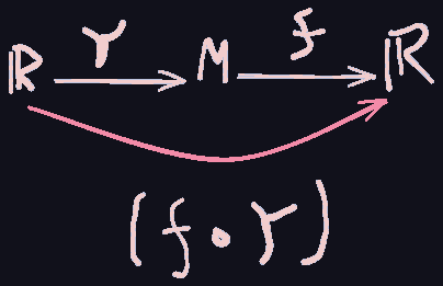
This whole definition of velocity is constrained to the fact that the curve $γ$ lives on a special manifold: one which itself lives in a nice 3D vector space.

So we need to reinvent our notion of velocity to generalise to a manifold where you don’t have the aforementioned luxuries. Enter a peculiar ant: It is direction-ally challenged, cannot measure distances, cannot add or subtract points on a manifold, or scale them, but despite all its flaws, it is very sensitive to temperature and is mathematically gifted. It can do calculus on the real numbers. Imagine now that this ant was moving on the curve $γ$ on the manifold instead of a particle. What you do is heat up this manifold in a specific way and give it a temperature function that takes any point $p$ in the manifold and gives that point’s absolute temperature $f (p)$ .

Now the ant here does something clever. Let’s say that at time $t = 0$ , it’s at the point $p$ , and you ask the ant, "What is your velocity here?" It first carefully records the temperature at point $p$ : $f (p)$ , then steps slightly ahead in time, say at $t + ϵ$ , lands on the point $p^{'}$ , and records the temperature $f (p^{'})$ . Then it tells you that $\frac{f (p^{'}) - f (p)}{ϵ}$ is a good approximation of its velocity. It basically avoided doing any operations on the manifold and instead did the operations on its sense of temperature!

But you tell the ant, "All that is clever, but ant, is your definition of velocity any good? Forget about working for general manifolds; does it even work for our special manifold which is in a nice 3D vector space? After all, what you’re giving me is a single number as the velocity for a point, but our velocity is actually a 3D vector."

The ant then says, "Not so fast, my friend. Actually, my definition of velocity depends on the temperature function that you give me. If you give me all possible temperature functions, I will define my velocity this way: if $γ$ is a curve from the real numbers $R$ to a manifold $M$ , and $f$ is any temperature function from the manifold $M$ to the reals $R$ , then the velocity at a point $p$ at time $t_{p}$ on the curve $γ$ is actually a function $v_{p, γ}$ that takes in a temperature function $f$ and returns the single-variable velocity $(f \circ γ)^{'} (t_{p})$ . That is, $v_{p, γ} : TEMPS \to R$ such that $v_{p, γ} (f) = (f \circ γ)^{'} (t_{p})$ ." (Here, $TEMPS$ is the set of all possible temperature functions from the manifold to the reals.)

You are a little frustrated with the ant’s definition. What is going on? Why should velocity (at a point and on a curve) be a function that takes in a temperature function from a manifold to the reals and spits out the derivative of the temperature it feels?

The ant says, "Don’t worry, I’ll prove that my definition works in your special little 3D manifold. In fact, I just want three special temperature functions. For one, I just want you to set the temperature of each point equal to its x-coordinate: $f_{x} (x, y, z) = x$ . For the other, I want you to set the temperature of each point equal to its y-coordinate: $f_{y} (x, y, z) = y$ , and similarly $f_{z} (x, y, z) = z$ . If you give me $f_{x}$ , I will use my definition of velocity and my sense of temperature alone and give you the correct x-component of the true velocity. Same for $f_{y}$ and $f_{z}$ ."

In the plots below, notice how when we use $f_{x}$ as the temperature function, our temperature-based velocity agrees with the x-component of the true velocity. Similarly for $f_{y}$ and $f_{z}$ :

You are now very impressed with the ant and accept its definition as a candidate.

Let’s walk through some math now. First, why is this definition a good candidate for the derivative/velocity of a curve on a general manifold?

Pasted image 20250522221949.png

The manifold $M$ in the middle is the problem; we can’t really do any arithmetic on points of $M$ itself in the general case. So we basically take each point in $M$ and assign a number (we were calling it temperature for intuitive reasons). And when you do that, you can do calculus on the numbers assigned to each point, but the derivative/velocity you get by doing that is dependent on how you assign these numbers—that is, it depends on $f$ . So you can think about $f$ giving a sense of direction, and $v_{γ, p} (f) = (f \circ γ)^{'} (t_{p})$ is analogous to a "directional derivative" at the point $p$ along the "direction" $f$ on the curve $γ$ .

And in the special case, if $M$ is actually a surface embedded in $R^{3}$ , for example, then the coordinate map $f_{x} (x, y, z) = x$ literally takes the point $p = (x, y, z)$ on the curve $γ$ and gives the x-coordinate.

In particular, if $γ (t_{p}) = p = (x (t_{p}), y (t_{p}), z (x (t_{p}), y (t_{p})))$ , where $z$ is the special manifold surface we’re using so far:

Manifold: z = \sin (0.5 x) \cos (0.5 y) \cdot 2 + e^{- 0.1 (x^{2} + y^{2})}

Then,

(f_{x} \circ γ) (t_{p}) = x (t_{p}) hence (f_{x} \circ γ)^{'} (t_{p}) = x^{'} (t_{p}) = {(\frac{d γ}{d t} (t_{p}))}_{x}

So we actually recover the x-component of the velocity on $γ$ . The same holds for the other coordinates too.

Mixing intuition and formalism is really messy, I know I haven't defined what a manifold is, or why you can't do arithmetic directly on the manifold and all that stuff, and I also know that I can do a better job and explaining stuff. Any improvements/suggestions are always welcome. Maybe one day I'll drop my raw formal notes on here, but that seems a little too lazy for now, besides, they're unedited and full of errors.